Nama:Bayu cahyadi
Kelas :TK 19 A
Npm :19316085
from notebook.services.config import ConfigManager
cm = ConfigManager()
cm.update('livereveal', {
'scroll': True,
'width': "100%",
'height': "100%",
})
{'height': '100%', 'scroll': True, 'width': '100%'}
5.1.
Introduction to Normal Distributions and
the Standard Normal Distribution
Definition of a Normal Distribution
x
A normal distribution is a continuous probability distribution for a random variable . The graph of a normal distribution is called the normal curve.
Properties of a Normal Distribution
A normal distribution has these properties:
1. The mean, median, and mode are equal.
2. The normal curve is bell-shaped and is symmetric about the mean. 3. The total area under the normal curve is equal to 1.
x
4. The normal curve approaches, but never touches, the -axis as it extends farther and farther away from the mean
μ − σ μ + σ
5. Between and (in the center of the curve), the graph curves downward. μ − σ μ + σ
The graph curves upward to the left of and to the right of . The ponts at which the curve changes from curving upward to curving downward are called inflection points.
Properties of a Normal Distribution
Properties of a Normal Distribution
A discrete probability distribution can be graphed with a histogram.
A continuous probability distribution, we can use a probability density function (pdf). A probability density function has two requirements:
1. the total area under the curve is equal to 1, and
2. the function can never be negative.
y =1
2σ2
Formula for pdf:
σ√2πe−(x−μ) /(2 )
Meand and Standard Deviation (recap)
Properties of a Normal Distribution [example 1]
Understanding Mean and Standard Deviation
1. Which normal curve has a greater mean?
2. Which normal curve has a greater standard deviation?
Properties of a Normal Distribution [solution]
x = 15
1. The line of symmetry of curve A occurs at .
x = 12
The line of symmetry of curve B occurs at .
So, curve A has a greater mean.
2. Curve B is more spread out than curve A.
So, curve B has a greater standard deviation.
Properties of a Normal Distribution [example 2]
Interpreting Graphs of Normal Distributions
The scaled test scores for the New York State Grade 8 Mathematics Test are normally distributed.
The normal curve shown below represents this distribution.
What is the mean test score? Estimate the standard deviation of this normal distribution.
Properties of a Normal Distribution [solution]
8
The scaled test scores for the New York State Grade Mathematics Test are normally 675 35
distributed with a mean of about and a standard deviation of about .
The Standard Normal Distribution
0 1
The normal distribution with a mean of and a standard deviation of is called the standard normal distribution.
z
The horizontal scale of the graph of the standard normal distribution corresponds to - scores.
value−mean
z = = standard_deviation
x−μ
σ
x z x
It is important that you know the difference between and . The random variable is sometimes called a raw score and represents values in a nonstandard normal distribution, z
whereas represents values in the standard normal distribution.
Properties of the Standard Normal Distribution
0 z z = −3.49
1. The cumulative area is close to for -scores close to . z
2. The cumulative area increases as the -scores increase.
z = 0 0.5
3. The cumulative area for is .
1 z z = 3.49
4. The cumulative area is close to for -scores close to .
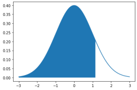
Using the Standard Normal Table and SciPy [example 3] z 1.15
Q1: Find the cumulative area that corresponds to a -score of
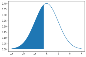
z −0.24
Q2: Find the cumulative area that corresponds to a -score of
Using the Standard Normal Table and SciPy [solution]
z 1.15
Q1: Find the cumulative area that corresponds to a -score of
z
Using -score calculator
Using SciPy
from scipy import stats
z_score = 1.15
p = stats.norm.cdf(z_score)
print(p)
0.8749280643628496
from scipy import stats
import numpy as np
import matplotlib.pyplot as plt
def draw_z_score(x, cond, mu=0, sigma=1):
y = stats.norm.pdf(x, mu, sigma)
z = x[cond]
plt.plot(x, y)
plt.fill_between(z, 0, stats.norm.pdf(z, mu, sigma))
plt.show()
x = np.arange(-3, 3, 0.001)
draw_z_score(x, x<z_score)


Tidak ada komentar:
Posting Komentar